Welcome to StonerPlots’s documentation!
Introduction
StonerPlots is a Python package designed to simplify the creation of publication-quality matplotlib figures. In particular, it is intended to produce plots that align with the style of common physics journals. StonerPlots also helps ensure consistency in matplotlib figures for reports, theses, and similar documentation.
The library originated as a fork of the scienceplots package by John D. Garrett.
Quickstart
Installation
StonerPlots can be installed using either pip or conda:
pip install stonerplots
Conda packages are available from the Anaconda channel phygbu:
conda install -c phygbu stonerplots
StonerPlots requires Python 3.10 or later and depends on matplotlib, which will be installed automatically. However, most example code also makes use of numpy, so you may wish to ensure it is installed.
Example
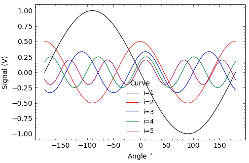
The easiest way to get started is by using the SavedFigure context manager. This automatically applies the requested styles and collects any new figures, saving them to disk:
import numpy as np
import matplotlib.pyplot as plt
from stonerplots import SavedFigure

# Generate example data
x = np.linspace(-np.pi, np.pi, 181)
fig_params = {"xlabel": r"Angle ($^\circ$)", "ylabel": "Signal (V)"}

# Save a styled figure
with SavedFigure("figures/example-1.png"):  # Replace 'figures' with your desired output path
    fig, ax = plt.subplots()
    for i in range(1, 6):
        ax.plot(x * 180 / np.pi, (1 / i) * np.sin(x * i + np.pi / i),
                marker="", label=f"i = {i}")
    ax.legend(title="Curve")
    ax.set(**fig_params)
In this example, the SavedFigure context manager applies the default “stoner” stylesheet and saves the figure as example-1.png. The file will be saved in the specified output directory (figures), which must already exist. Ensure to adjust the path as needed for your use case.
Sections
Explore various aspects of StonerPlots through the following sections:
Indices and tables
Explore further using the indices and search functionality provided below: