Stoner Plots Style Gallery¶

1. Default Styles¶

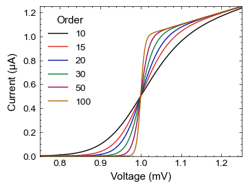
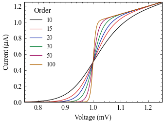
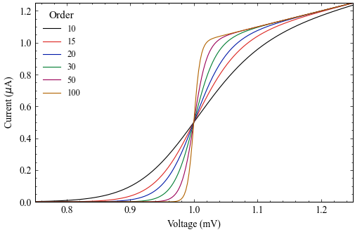
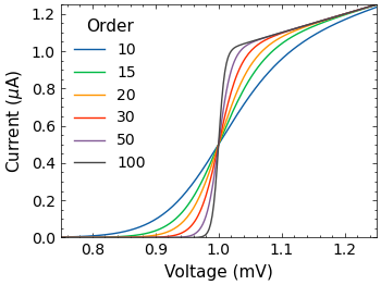
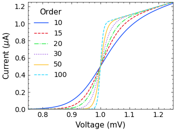
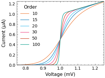
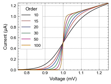
Basic stoner style:¶

The basic stylesheet is the stoner stylesheet:

with SavedFigure(figures / "fig01a.png", style=["stoner"], autoclose=True):
    fig, ax = plt.subplots()
    for p in [10, 15, 20, 30, 50, 100]:
        ax.plot(x, model(x, p), label=p, marker="")
    ax.legend(title="Order")
    ax.autoscale(tight=True)
    ax.set(**pparam)

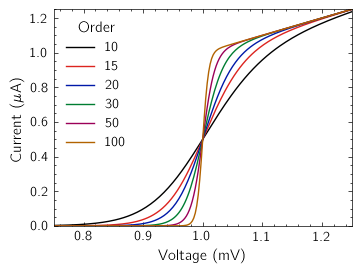
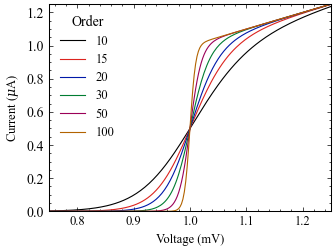
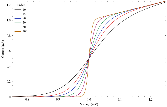
Example figure formatted with the 'stoner' style sheet.

LaTeX Rendering¶

The basic stoner style uses matplotlib’s built-in emulation of LaTeX to render mathematical expressions. Use the latex modifier to turn on LaTeX rendering of text and maths:

with SavedFigure(figures / "fig01b.png", style=["stoner", "latex"], autoclose=True):
    fig, ax = plt.subplots()
    for p in [10, 15, 20, 30, 50, 100]:
        ax.plot(x, model(x, p), label=p, marker="")
    ax.legend(title="Order")
    ax.autoscale(tight=True)
    ax.set(**pparam)

2. Journal Formats¶

There are specific stylesheets for producing plots at the correct size and style for some common Physics journals.

Using styles [“stoner”, “ieee”]	Using styles [“stoner”, “aps”]
Using styles [“stoner”, “aip”]	Using styles [“stoner”, “iop”]
Using styles [“stoner”, “nature”]	Using styles [“stoner”, “aaas-science”]
Using styles [“stoner”, “aps”, “aps1.5”]
Using styles [“stoner”, “aps”, “aps2”]
Using styles [“stoner”, “thesis”]
Using styles [“stoner”, “thesis”] and MultiPanel with manual adjust_figsize=(0, -0.25)

3. Different Plot Types¶

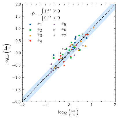
There is a scatter plot style that sets up for doing scatter plots.

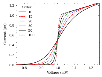
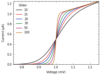
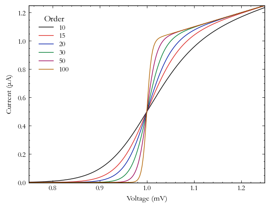
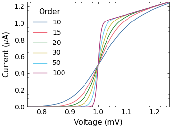
4. Different Colour Schemes¶

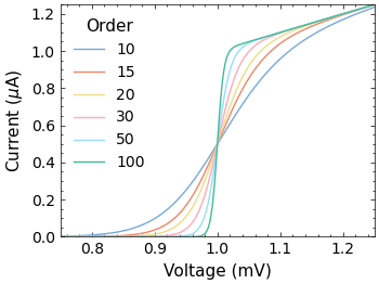
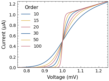
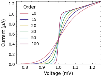
Using styles [“stoner”, “std-colours”]	Using styles [“stoner”, “bright”]
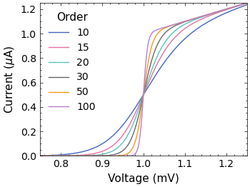
Using styles [“stoner”, “high-contrast”]	Using styles [“stoner”, “high-vis”]
Using styles [“stoner”, “light”]	Using styles [“stoner”, “muted”]
Using styles [“stoner”, “retro”]	Using styles [“stoner”, “vibrant”]
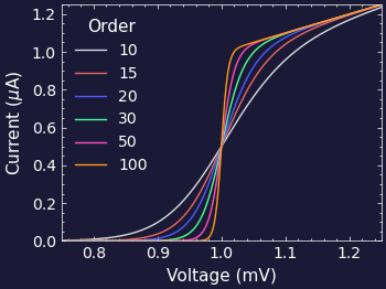
Using styles [“stoner”, “stoner-dark”]

In addition to switching the background to TfL Night Service black, the stoner-dark scheme also switches the colour cycler to use the slightly lighter Tube Map 50% shade colours.

5. Different Formats¶

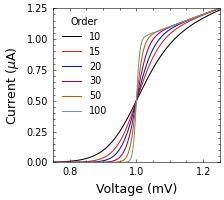
Notebooks¶

The notebook style is designed for Jupyter Notebooks.

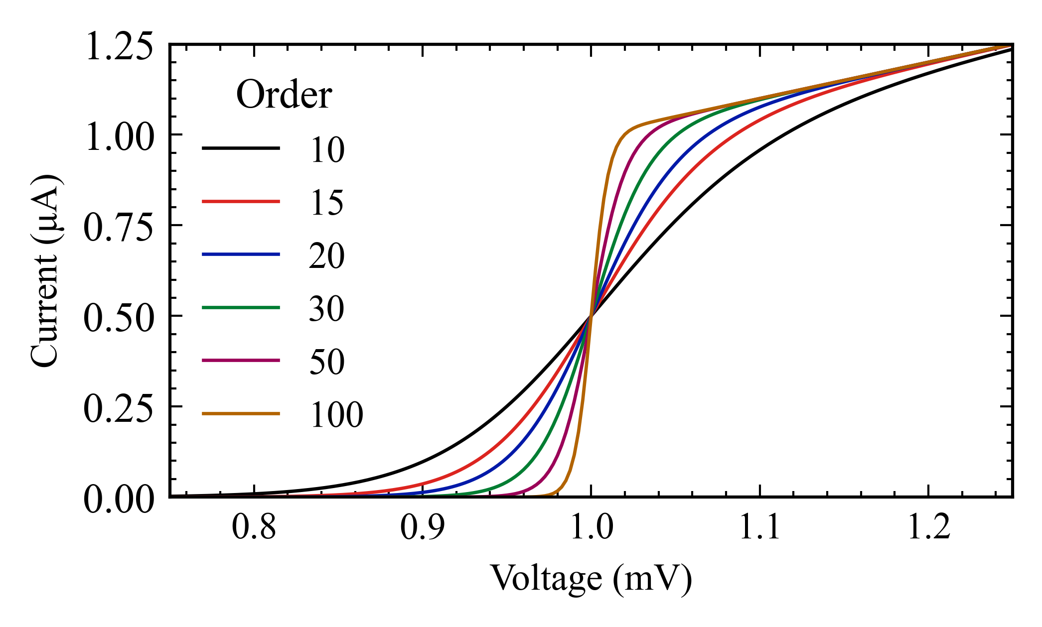
Posters¶

The poster style makes everything bigger for printing onto an A0 poster. Should be used in combination with hi-res for final printing.

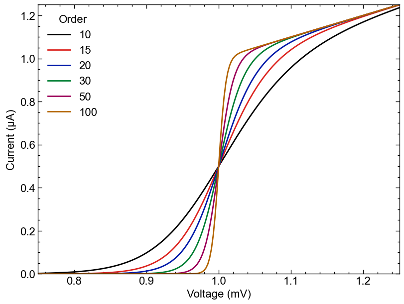
Presentations¶

The presentation style switches to a larger style, designed for use as a single graph on a PowerPoint presentation.

There is a presentation_sm style for when you want two plots on a slide.

The stoner_dark style does make everything look a bit heavier and bolder, so the presentation_dark lightens everything up.

Higher Resolution Modes¶

In general, for printed media, you should pick a vector format for saving figures - such as eps, svg or pdf. If this is not feasible and a bitmapped image is needed, then a higher dpi is required. This can be done by using the med-res or hi-res styles.

med-res Style¶

hi-res Style¶

6. Miscellaneous Tweaks¶

The grid style adds an axes grid to the plot.

This was produced with the style [“stoner”, “grid”].

7. Insets and Multi-panel plots¶

Double Y-Axis Plots¶

The stonerplots.DoubleYAxis context manager can be used to add a new set of axes as a second y-axis on the right hand side of the existing axes’ frame. The left and right y-axes can be coloured differently and the legend of both sets of axes combined.

Inset Plots¶

The stonerplots.InsetPlot context manager can be used to add a new set of axes as an inset to a plot. It can automatically position the inset(s) to keep clear of each other and the parent plot features.

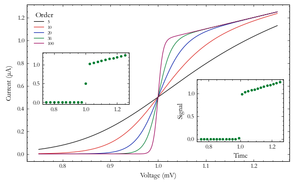
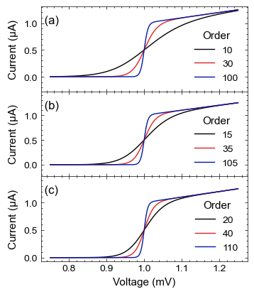
Plot with an inset in lower right corner and a second in the middle left side.

Stacked Sub-plots¶

When you want to compare several variables against a common independent variable, stacking the plots can be useful. The stonerplots.StackVertical context manager can be used for this.

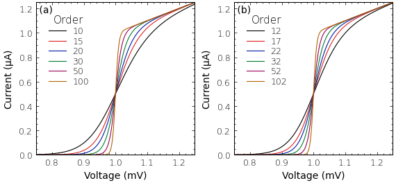
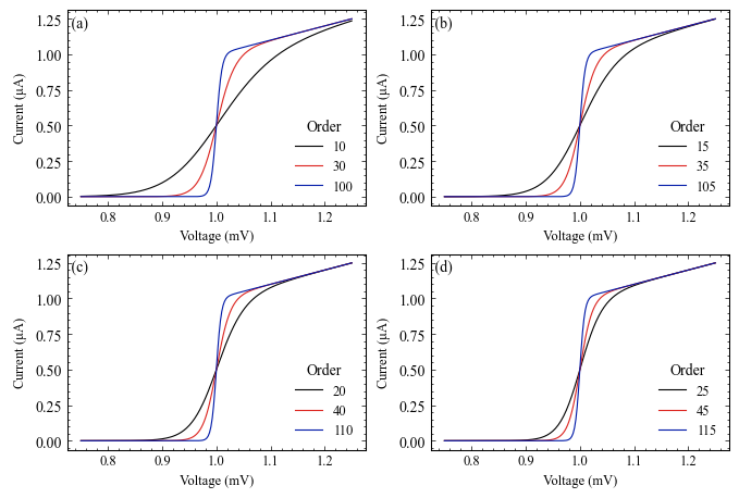
MultiPanel Sub-plots¶

Where a figure just needs to show a collection of related datasets, a multi-panel figure with sub-plots is a good option. The stonerplots.MultiPanel context manager makes this a bit easier.

Consistent Axes Formatting¶

The stonerplots.PlotLabeller context manager can adjust the axes label formatting for multiple figures.