MultiPanel Context Manager

Another common requirement when writing papers and theses is to create a figure with several distinct panels showing different (related) datasets. In this case, the MultiPanel context manager works in a very analogous way to the StackVertical context manager:

with MultiPanel((2, 2)) as axes:
    for ax, x, y in zip(axes, [x1, x2, x3, x4], [y1, y2, y3, y4]):
        ax.plot(x, y)

The only required parameter is the number of panels to show. This can be either - a tuple of (n_rows, n_cols), or - an integer specifying a number of columns (number of rows is assumed to be one in this case), or - a list of [row_1_plots, row_2_plots, …] to specify a different number of plots on each row.

Optional Parameters

The figure, sharex, sharey and label_panels parameters work exactly as for the StackVertical context manager described above, except that the default is not to share any axes - see Stacked Plots<stackvertical> for more details.

The adjust_figsize parameter allows you to specify a tuple defining distinct expansion factors for width and height. The default value is to expand the width by exactly the number of columns and the height by the height of one row + 80% of additional rows. Since full-page width figures are more than double a single column, it may be useful to do something like:

with SavedFigure("example.png", style=["stoner", "aip", "aip2"]):
    with MultiPanel((1, 2), adjust_figsize=(0, 0.12)) as axes:
        for ax, x, y in zip(axes, [x1, x2, x3, x4], [y1, y2, y3, y4]):
            ax.plot(x, y)

To create a figure that spans the full width and is two single plots tall.

For the figure below (from the style gallery), the adjust_figsize was set to (0, -0.25), meaning that width was preserved, and height was reduced by a factor of -25%. Whilst a positive expansion factor is applied to the additional rows, the negative value is applied to the original figure size. (The logic here is that the times you need to shrink the original figure size is when the final aspect ratio will be higher than the original figure).

Use with Presentation Style

Combining MultiPanel with the presentation stylesheet is a good way to prepare multiple graphs for a single slide. The default behaviour of the adjust_figsize is unhelpful as the presentation stylesheet already sets a good figure size to use. You may also not want to label the individual panels:

with SavedFigure("fig7e.svg", style="stoner,presentation"):
    fig = plt.figure()
    with MultiPanel((2, 2), adjust_figsize=False, label_panels=False) as axes:
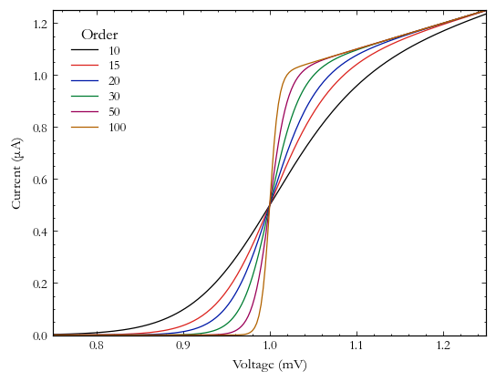
        for ix, ax in enumerate(axes):
            for p in [10, 30, 100]:
                ax.plot(x, model(x, p + ix * 5), label=p + ix * 5, marker="")
            ...

Different Numbers of Plots on Each Row

MultiPanel can also be used to create arrangements where there are different numbers of subplots on different rows on the figure. For example, if you want to have three subplots and they don’t conveniently fit on a single row, you might have 1 and then 2 plots, or 2 and then 1 plot. This can be achieved by using a list of plots per row as the first argument in conjunction with an optional same_aspect:

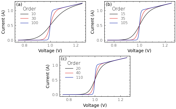
with SavedFigure("3-plot.png", style="stoner,thesis"):
    fig = plt.figure("tri-plot")
    with MultiPanel([2, 1], adjust_figsize=False) as axes:
        for ix, ax in enumerate(axes):
            ax.plot(x_data[ix], y_data[ix], marker="")
            ...

By default, MultiPanel will adjust the aspect to match the narrowest figure unless you specify same_aspect to be False, or give width_ratios or height_ratios to manually change the aspect ratios of the plots.

With the optional transpose argument, the MultiPanel will create a grid of plots, with each column potentially containing a different number of rows:

with SavedFigure("3-plot.png", style="stoner,thesis"):
    fig = plt.figure("tri-plot-transpose")
    with MultiPanel([1, 2], transpose=True, adjust_figsize=(0, -0.25)) as axes:
        for ix, ax in enumerate(axes):
            ax.plot(x_data[ix], y_data[ix], marker="")
            ...

Using the Context Manager Variable

The object returned when you enter the context exposes several useful bits of functionality. Firstly, if you iterate over the object it will return the individual plot axes - but it will also set pyplot’s current axes so that the matplotlib.pyplot interactive interface will work and switch between the plots as it iterates:

fig = plt.figure("tri-plot-b")
with MultiPanel([2, 1], adjust_figsize=False) as panels:
    for ix, _ in enumerate(panels):
        plt.plot(x_data[ix], y_data[ix], marker="")
        plt.xlabel("Voltage (mV)")
        plt.ylabel("Current ($\\mu$A)")
        ...

You can also access the underlying list or array of matplotlib.axes.Axes instances with the axes attribute and the matplotlib.gridspec.GridSpec used for the multi-panel plot. Indexing the context manager variable can also give access to the individual plots (or rows of plots if a single index is given):

fig = plt.figure("tri-plot-c")
with MultiPanel([2, 1], adjust_figsize=False) as panels:
    ax = panels[0, 0]  # Also set ax to be current axes
    plt.plot(x, y, ...)