StackVertical Context Manager
When comparing several quantities that have a common independent variable, using a sequence of vertically stacked plots can be effective. Typically, each sub-plot is positioned so that the top x-axis of one panel is the bottom x-axis of the one above, and only the bottom x-axis of the whole stack is labelled.
Although matplotlib’s built-in features to make multiple plots on a grid have been improved in recent releases, it is
still quite complex, and getting the plots to be adjacent, whilst also not having the labels clash, is challenging.
StackVertical is a context manager designed to make this easier:
with StackVertical(3) as axes:
    for ax, y in zip(axes, [y_data1, y_data2, y_data3]):
        ax.plot(x, y)
The only required parameter to StackVertical is the number of plots to stack vertically. It then returns a
list of the matplotlib.axes.Axes for each subplot - the first set of axes being the top plot and the last
being the bottom.
When the context manager exits, it adjusts the y-axis limits to ensure the tick markers do not interfere and reduces the spacing between the plots to zero so that they are adjacent.
Adjusting the Figure Size for the Stack
By default, StackVertical will look at the current figure to work out its dimensions and will then assume that
this is the correct size for a single plot. It will then adjust the figure height to accommodate the additional stacked
plots. The equation used for this is:
with \(f\) being a fraction of the old plot size set by the adjust_figsize parameter to StackVertical.
If this is left at the default value of True, then \(f\) is set to 0.6 and reduced to 0 if adjust_figsize is
False.
Typically, stacked plots have a bigger aspect ratio (width:height) than a single plot:
with StackVertical(3, adjust_figsize=0.5) as axes:
    for ax, y in zip(axes, [y_data1, y_data2, y_data3]):
        ax.plot(x, y)
Labelling the Panels
A common requirement of a multi-panel figure is to label the individual sets of axes (a), (b)… or similar. This is
supported by the label_panels parameter. If this takes the value True, then each set of axes is labelled ‘(a)’,
‘(b)’ and so forth. For additional control, the parameter can also take a string similar to the format used in
SavedFigure above. Placeholders such as {Alpha} or {roman} can be used to indicate the axes number:
with StackVertical(3, label_panels=True) as axes:
    for ax, y in zip(axes, [y_data1, y_data2, y_data3]):
        ax.plot(x, y)
Some journals, e.g. Science, also want the label to be in bold font, and StackVertical supports passing the
font keyword arguments to control the font size and appearance:
with StackVertical(3, label_panels='{Alpha}', fontweight='bold') as axes:
    for ax, y in zip(axes, [y_data1, y_data2, y_data3]):
        ax.plot(x, y)
Specifying a Figure
The default is to use the current matplotlib figure, but by passing the figure parameter into the StackVertical
context manager, it will use that figure instead:
with StackVertical(3, figure=2) as axes:
    for ax, y in zip(axes, [y_data1, y_data2, y_data3]):
        ax.plot(x, y)
The figure parameter can be either a matplotlib.figure.Figure or a figure number or figure label. Within
the context manager, the current figure is set to be the figure specified by the figure parameter. The previously
active figure is reset as active when the context manager exits.
Not Joining the Plots
Although it is envisaged that the main use of the StackVertical context manager is to make plots with shared x-axes
and sitting adjacent to each other, setting the joined parameter to False will stop the post-plotting resizing and
adjustment of the y-limits and therefore set the plots as separate entities:
with StackVertical(3, joined=False) as axes:
    for ax, y in zip(axes, [y_data1, y_data2, y_data3]):
        ax.plot(x, y)
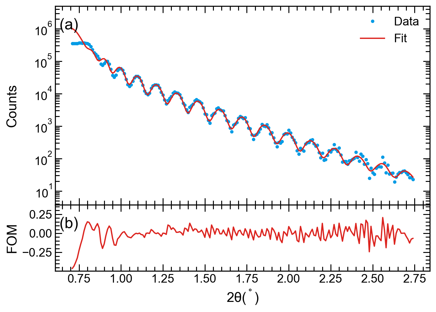
Advanced Usage
You can also pass a heights_ratio into the StackVertical to control the relative heights of the plots. A use
for this is when you have a primary set of data and a related subsidiary data set. For example, in fitting a set of data,
one might show the data and fit on the main panel and the residuals or a figure of merit in a secondary panel:
import numpy as np
import matplotlib.pyplot as plt
from stonerplots import SavedFigure, StackVertical

# Prepare data assuming a data format of x, y_fit, y_obs
data = np.genfromtxt(Path(__file__).parent.parent / "data" / "xrr.dat")
x = data[:, 0]
fit = data[:, 1]
measured = data[:, 2]
fom = np.log10(measured) - np.log10(fit)

# Set up the scales, labels etc for the two panels.
main_props = {"ylabel": "Counts", "yscale": "log", "ylim": (10, 5E6)}
residual_props = {"xlabel": r"2$\theta (^\circ)$", "ylabel": "FOM"}

# This is stonerplots context managers at work
with SavedFigure(figures / "genx_plot.png", style=["stoner", "presentation"], autoclose=True):
    plt.figure()
    with StackVertical(2, adjust_figsize=False, heights_ratio=[3, 1]) as axes:
        main, residual = axes
        main.plot(x, measured, linestyle="", marker=".", label="Data", c="victoria")
        main.plot(x, fit, marker="", label="Fit", c="central")
        main.set(**main_props)
        main.legend()
        residual.plot(x, fom, marker="", c="central")
        residual.set(**residual_props)
(The data in the example is a rather poor fit to some X-ray reflectivity data with the GenX software). It produces the following output: